唔係連點樣用 AI 提問都唔識啩
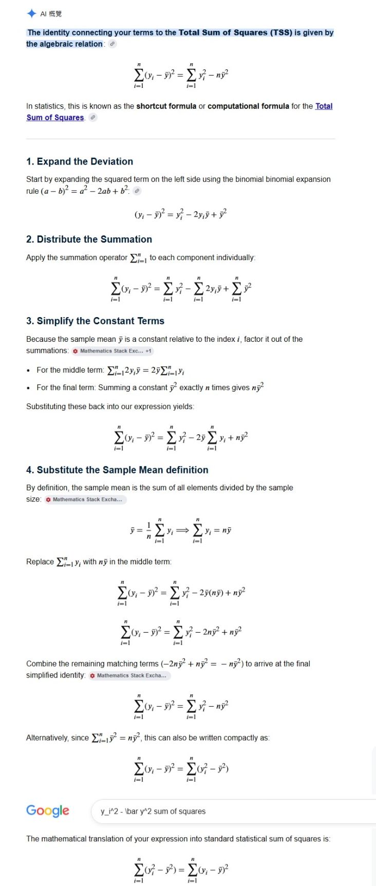
Properties of Variance
-
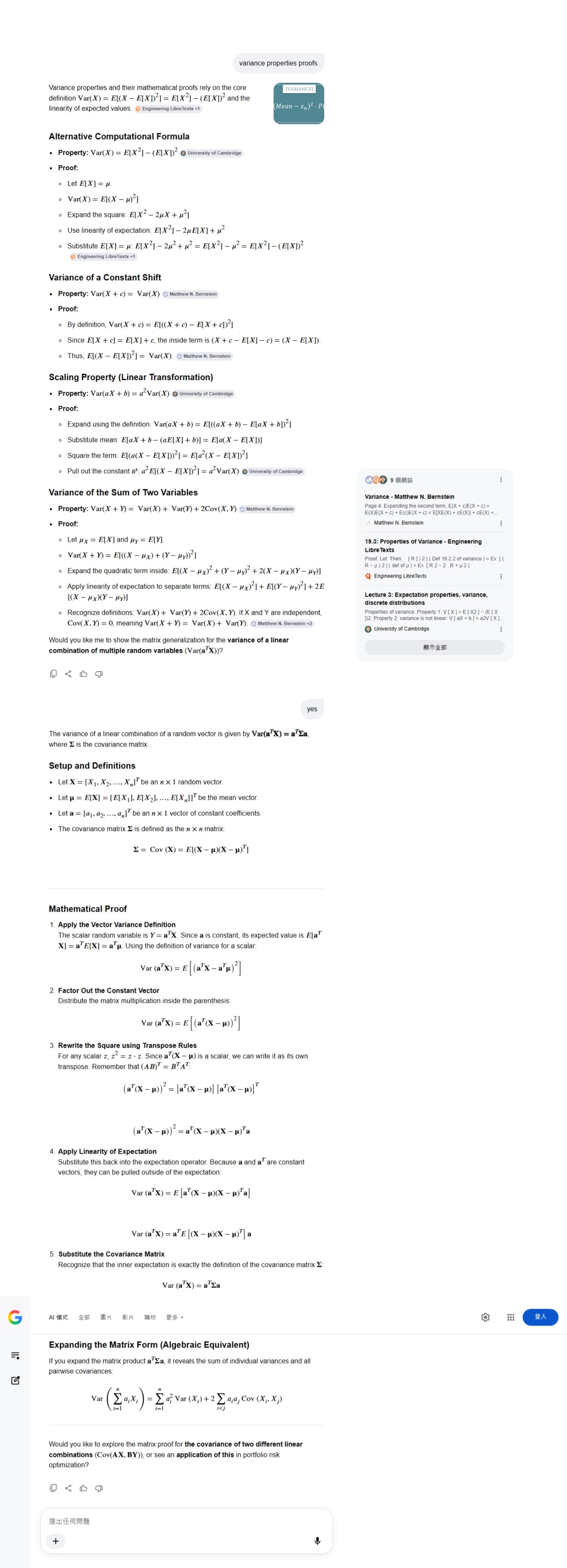
Non-negativity: Var(X) ≥ 0. Variance is always zero or positive because it is the expectation of squared deviations.
-
Constant shift: Var(X + c) = Var(X) for any constant c. Adding a fixed value shifts the data but does not change the spread.
-
Scaling by a constant: Var(aX) = a² Var(X). Scaling a variable multiplies its variance by the square of that constant.
-
Sum of independent variables: If X and Y are independent, then Var(X + Y) = Var(X) + Var(Y).
-
General sum formula: Var(X + Y) = Var(X) + Var(Y) + 2Cov(X, Y).
Properties of Covariance
-
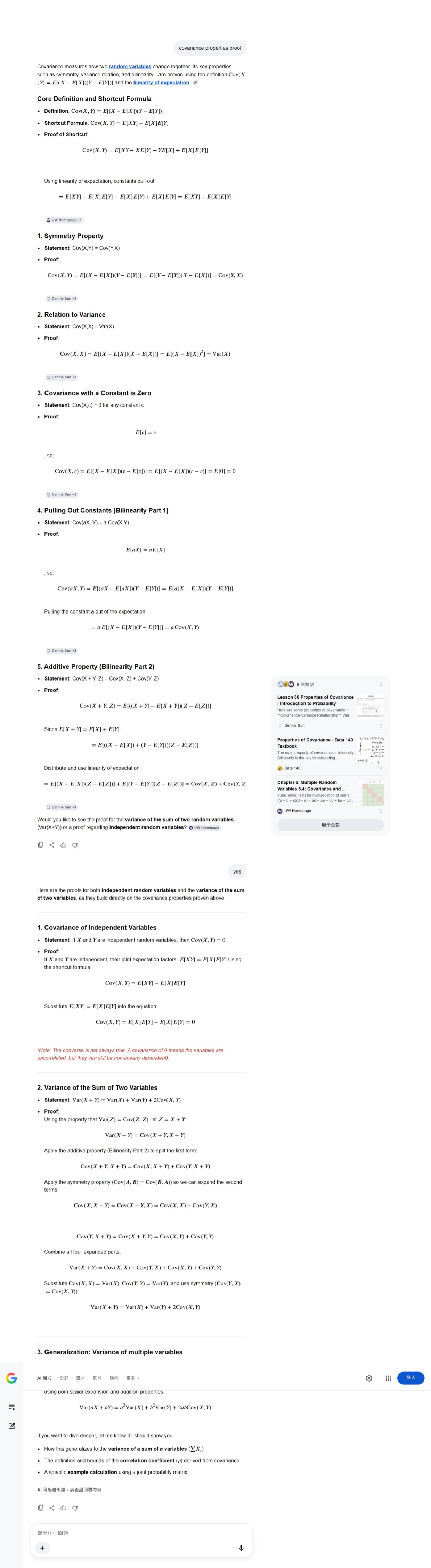
Symmetry: Cov(X, Y) = Cov(Y, X). The order of variables does not change the result.
-
Relationship to variance: Cov(X, X) = Var(X). The covariance of a variable with itself equals its variance.
-
Constants and zero covariance: Cov(X, c) = 0 for any constant c. A constant has no variation to share with X.
-
Bilinearity (Pulling out constants): Cov(aX + b, cY + d) = acCov(X, Y). Constants inside the addition vanish, and multipliers factor right out.
-
Additivity / Distributive property: Cov(X + Y, Z) = Cov(X, Z) + Cov(Y, Z).
-
Independence implies zero covariance: If X and Y are independent, Cov(X, Y) = 0. Note that a covariance of zero does not always mean they are fully independent, only that there is no linear relationship.
連呢啲常識都要等人餵就咪撚學人讀經濟
Here are the formal proofs for continuous random variables using probability density functions (PDF), where f_X(x) represents the PDF of X and the integrals evaluate from -\infty to \infty . [1, 2]
- Computational Formula Proof (Var(X) = E[X^2] - (E[X])^2)
- Start with the continuous integral definition of variance:
Var(X)=\int _{-\infty }^{\infty }(x-\mu )^{2}f_{X}(x)\,dx [1] - Expand the polynomial inside the integrand:
\int _{-\infty }^{\infty }(x^{2}-2\mu x+\mu ^{2})f_{X}(x)\,dx - Split the integral into three separate terms:
\int _{-\infty }^{\infty }x^{2}f_{X}(x)\,dx-\int _{-\infty }^{\infty }2\mu xf_{X}(x)\,dx+\int _{-\infty }^{\infty }\mu ^{2}f_{X}(x)\,dx - Factor out the constants (\mu is a fixed scalar value):
\int _{-\infty }^{\infty }x^{2}f_{X}(x)\,dx-2\mu \int _{-\infty }^{\infty }xf_{X}(x)\,dx+\mu ^{2}\int _{-\infty }^{\infty }f_{X}(x)\,dx - Apply fundamental calculus and probability axioms:
- \int_{-\infty}^{\infty} x^2 f_X(x) \, dx = E[X^2]
- \int_{-\infty}^{\infty} x f_X(x) \, dx = \mu
- \int_{-\infty}^{\infty} f_X(x) \, dx = 1 (Total probability rule)
- Substitute these values back into the expression:
E[X^{2}]-2\mu (\mu )+\mu ^{2}(1)=E[X^{2}]-2\mu ^{2}+\mu ^{2}=E[X^{2}]-\mu ^{2} [1] - Re-substitute \mu = E[X] to finish:
Var(X)=E[X^{2}]-(E[X])^{2}
- Linear Scaling Proof (Var(aX + b) = a^2 Var(X))
- Let Y = aX + b. Find the expected value E[Y] first:
E[aX+b]=\int _{-\infty }^{\infty }(ax+b)f_{X}(x)\,dx=a\int _{-\infty }^{\infty }xf_{X}(x)\,dx+b\int _{-\infty }^{\infty }f_{X}(x)\,dx=a\mu +b - Set up the variance integral for the transformed variable:
Var(aX+b)=\int _{-\infty }^{\infty }\left[(ax+b)-(a\mu +b)\right]^{2}f_{X}(x)\,dx - Simplify the terms inside the square bracket (b cancels out):
\int _{-\infty }^{\infty }(ax-a\mu )^{2}f_{X}(x)\,dx=\int _{-\infty }^{\infty }a^{2}(x-\mu )^{2}f_{X}(x)\,dx - Pull the constant a^{2} outside the integral operator:
a^{2}\int _{-\infty }^{\infty }(x-\mu )^{2}f_{X}(x)\,dx - Recognize the remaining integral as the definition of Var(X):
Var(aX+b)=a^{2}Var(X)
- Independent Additivity Proof (Var(X + Y) = Var(X) + Var(Y))
- Let X and Y be independent continuous variables with joint PDF f_{X,Y}(x,y) = f_X(x)f_Y(y).
- Let \mu_X = E[X] and \mu_Y = E[Y]. The variance of their sum uses a double integral:
Var(X+Y)=\int _{-\infty }^{\infty }\int _{-\infty }^{\infty }\left[(x+y)-(\mu _{X}+\mu _{Y})\right]^{2}f_{X,Y}(x,y)\,dx\,dy - Group the terms by variable type inside the squared bracket:
\int _{-\infty }^{\infty }\int _{-\infty }^{\infty }\left[(x-\mu _{X})+(y-\mu _{Y})\right]^{2}f_{X,Y}(x,y)\,dx\,dy - Expand the binomial expression:
\int _{-\infty }^{\infty }\int _{-\infty }^{\infty }\left[(x-\mu _{X})^{2}+2(x-\mu _{X})(y-\mu _{Y})+(y-\mu _{Y})^{2}\right]f_{X,Y}(x,y)\,dx\,dy - Split this into three distinct double integrals. Due to independence, the middle term simplifies:
2\int _{-\infty }^{\infty }\int _{-\infty }^{\infty }(x-\mu _{X})(y-\mu _{Y})f_{X}(x)f_{Y}(y)\,dx\,dy=2\left[\int _{-\infty }^{\infty }(x-\mu _{X})f_{X}(x)\,dx\right]\left[\int _{-\infty }^{\infty }(y-\mu _{Y})f_{Y}(y)\,dy\right] - Because \int_{-\infty}^{\infty} (x - \mu_X) f_X(x) \, dx = \mu_X - \mu_X = 0, the entire cross-term evaluates to 0.
- Evaluate the remaining two outer terms using marginal distributions:
\int _{-\infty }^{\infty }(x-\mu _{X})^{2}f_{X}(x)\,dx+\int _{-\infty }^{\infty }(y-\mu _{Y})^{2}f_{Y}(y)\,dy=Var(X)+Var(Y) [1]
The shortcut formula for covariance, \text{Cov}(X,Y) = E[XY] - E[X]E[Y], is proven for continuous random variables by expanding the definition via expected value integrals and applying the linearity property of integrals. [1, 2, 3, 4]
Proof Setup and Expansion
-
Let X and Y have a joint probability density function f(x,y).
-
Let the expected values be \mu_X = E[X] and \mu_Y = E[Y].
-
By definition, covariance is \text{Cov}(X,Y) = E[(X - \mu_X)(Y - \mu_Y)].
-
Write this expected value as a double integral:
\text{Cov}(X,Y)=\int _{-\infty }^{\infty }\int _{-\infty }^{\infty }(x-\mu _{X})(y-\mu _{Y})f(x,y)\,dx\,dy [1, 2, 3, 4]
Expanding the Integrand
-
Multiply the terms inside the integral:
(x-\mu _{X})(y-\mu _{Y})=xy-x\mu _{Y}-y\mu _{X}+\mu _{X}\mu _{Y} -
Substitute this expanded form back into the double integral:
\text{Cov}(X,Y)=\int _{-\infty }^{\infty }\int _{-\infty }^{\infty }(xy-x\mu _{Y}-y\mu _{X}+\mu _{X}\mu _{Y})f(x,y)\,dx\,dy [1, 2]
Splitting and Distributing the Integral
- Split the double integral into four separate integrals using linearity:
\text{Cov}(X,Y)=\int _{-\infty }^{\infty }\int _{-\infty }^{\infty }xyf(x,y)\,dx\,dy-\mu _{Y}\int _{-\infty }^{\infty }\int _{-\infty }^{\infty }xf(x,y)\,dx\,dy-\mu _{X}\int _{-\infty }^{\infty }\int _{-\infty }^{\infty }yf(x,y)\,dx\,dy+\mu _{X}\mu _{Y}\int _{-\infty }^{\infty }\int _{-\infty }^{\infty }f(x,y)\,dx\,dy [1]
Evaluating the Integral Components
-
The first term is the definition of E[XY]:
\int _{-\infty }^{\infty }\int _{-\infty }^{\infty }xyf(x,y)\,dx\,dy=E[XY] -
For the second term, factor out \mu _{Y} and recognize that \int_{-\infty}^{\infty} x f(x,y) \,dx\,dy = \mu_X (marginal expectation):
\mu _{Y}\int _{-\infty }^{\infty }x\left[\int _{-\infty }^{\infty }f(x,y)\,dy\right]dx=\mu _{Y}E[X]=\mu _{Y}\mu _{X}=E[X]E[Y] -
For the third term, factor out \mu _{X} similarly:
\mu _{X}\int _{-\infty }^{\infty }y\left[\int _{-\infty }^{\infty }f(x,y)\,dx\right]dy=\mu _{X}E[Y]=\mu _{X}\mu _{Y}=E[X]E[Y] -
For the fourth term, the total integral of the joint density f(x,y) equals 1:
\mu _{X}\mu _{Y}\int _{-\infty }^{\infty }\int _{-\infty }^{\infty }f(x,y)\,dx\,dy=\mu _{X}\mu _{Y}(1)=E[X]E[Y]
[1, 2]
Final Simplification
-
Combine all evaluated parts:
\text{Cov}(X,Y)=E[XY]-E[X]E[Y]-E[X]E[Y]+E[X]E[Y] -
Cancel out the matching terms to finish the proof:
\text{Cov}(X,Y)=E[XY]-E[X]E[Y]
For a random vector \mathbf{X} with mean \boldsymbol{\mu} = E[\mathbf{X}], the covariance matrix is defined as \boldsymbol{\Sigma} = E[(\mathbf{X} - \boldsymbol{\mu})(\mathbf{X} - \boldsymbol{\mu})^T]. Under a linear transformation \mathbf{Y} = \mathbf{A}\mathbf{X} + \mathbf{b} (with constant matrix \mathbf{A} and vector \mathbf{b}), the new covariance matrix is \boldsymbol{\Sigma}_{\mathbf{Y}} = \mathbf{A} \boldsymbol{\Sigma} \mathbf{A}^T. [1, 2, 3]
Proof of Linear Transformation Property
-
Find the mean of \mathbf{Y}:
\mathbfit{\mu }_{\mathbf{Y}}=E[\mathbf{AX}+\mathbf{b}]=\mathbf{A}E[\mathbf{X}]+\mathbf{b}=\mathbf{A}\mathbfit{\mu }+\mathbf{b} -
Substitute into the covariance definition:
\mathbfit{\Sigma }_{\mathbf{Y}}=E[(\mathbf{Y}-\mathbfit{\mu }_{\mathbf{Y}})(\mathbf{Y}-\mathbfit{\mu }_{\mathbf{Y}})^{T}] -
Replace \mathbf{Y} and \mathbfit{\mu }_{\mathbf{Y}} with their expanded forms:
\mathbf{Y}-\mathbfit{\mu }_{\mathbf{Y}}=(\mathbf{AX}+\mathbf{b})-(\mathbf{A}\mathbfit{\mu }+\mathbf{b})=\mathbf{A}(\mathbf{X}-\mathbfit{\mu }) -
Insert this back into the expectation:
\mathbfit{\Sigma }_{\mathbf{Y}}=E[\mathbf{A}(\mathbf{X}-\mathbfit{\mu })(\mathbf{A}(\mathbf{X}-\mathbfit{\mu }))^{T}] -
Use the transpose rule (\mathbf{M}\mathbf{N})^T = \mathbf{N}^T \mathbf{M}^T:
{}^{\mathbf{A}(\mathbf{X}-\mathbfit{\mu })^{T}=(\mathbf{X}-\mathbfit{\mu })^{T}\mathbf{A}^{T}} -
Factor out the constant matrix \mathbf{A} and \mathbf{A}^{T} using linearity of expectation:
\mathbfit{\Sigma }_{\mathbf{Y}}=\mathbf{A}E[(\mathbf{X}-\mathbfit{\mu })(\mathbf{X}-\mathbfit{\mu })^{T}]\mathbf{A}^{T}=\mathbf{A}\mathbfit{\Sigma }\mathbf{A}^{T}
[1, 2]
Proof of Symmetry Property
-
Recall definition: \boldsymbol{\Sigma} = E[(\mathbf{X} - \boldsymbol{\mu})(\mathbf{X} - \boldsymbol{\mu})^T]
-
Take the transpose of the covariance matrix:
\mathbfit{\Sigma }^{T}=(E[(\mathbf{X}-\mathbfit{\mu })(\mathbf{X}-\mathbfit{\mu })^{T}])^{T} -
Transpose of an expected value is the expected value of the transpose:
\mathbfit{\Sigma }^{T}=E[((\mathbf{X}-\mathbfit{\mu })(\mathbf{X}-\mathbfit{\mu })^{T})^{T}] -
Reverse the inner product order:
((\mathbf{X}-\mathbfit{\mu })^{T})^{T}(\mathbf{X}-\mathbfit{\mu })^{T}=(\mathbf{X}-\mathbfit{\mu })(\mathbf{X}-\mathbfit{\mu })^{T} -
Result: \boldsymbol{\Sigma}^T = \boldsymbol{\Sigma}, proving it is symmetric. [1, 2]
Proof of Positive Semi-Definite Property
-
Take a non-zero constant vector \mathbf{v}:
\mathbf{v}^{T}\mathbfit{\Sigma }\mathbf{v}=\mathbf{v}^{T}E[(\mathbf{X}-\mathbfit{\mu })(\mathbf{X}-\mathbfit{\mu })^{T}]\mathbf{v} -
Move \mathbf{v}^{T} and \mathbf{v} inside the linear expectation operator:
\mathbf{v}^{T}\mathbfit{\Sigma }\mathbf{v}=E[\mathbf{v}^{T}(\mathbf{X}-\mathbfit{\mu })(\mathbf{X}-\mathbfit{\mu })^{T}\mathbf{v}] -
Group terms as a scalar square: Note that \mathbf{v}^T (\mathbf{X} - \boldsymbol{\mu}) is a scalar, and its transpose is (\mathbf{X} - \boldsymbol{\mu})^T \mathbf{v}.
\mathbf{v}^{T}\mathbfit{\Sigma }\mathbf{v}=E[(\mathbf{v}^{T}(\mathbf{X}-\mathbfit{\mu }))^{2}] -
Conclusion: The expected value of a squared real random variable is always greater than or equal to zero, so \mathbf{v}^T \boldsymbol{\Sigma} \mathbf{v} \ge 0, meaning \mathbfit{\Sigma } is positive semi-definite.
For two random vectors \mathbf{X} (dimension m \times 1) and \mathbf{Y} (dimension n \times 1) with means \mathbfit{\mu }_{\mathbf{X}} and \mathbfit{\mu }_{\mathbf{Y}}, the cross-covariance matrix \boldsymbol{\Sigma}_{\mathbf{X}\mathbf{Y}} = \text{Cov}(\mathbf{X}, \mathbf{Y}) is defined as the m \times n matrix E[(\mathbf{X} - \boldsymbol{\mu}_{\mathbf{X}})(\mathbf{Y} - \boldsymbol{\mu}_{\mathbf{Y}})^T]. Under linear transformations \mathbf{U} = \mathbf{A}\mathbf{X} + \mathbf{b} and \mathbf{V} = \mathbf{C}\mathbf{Y} + \mathbf{d}, the transformed cross-covariance matrix is \text{Cov}(\mathbf{U}, \mathbf{V}) = \mathbf{A} \text{Cov}(\mathbf{X}, \mathbf{Y}) \mathbf{C}^T.
Proof of Linear Transformation Property
- Find the transformed means:
\mathbfit{\mu }_{\mathbf{U}}=\mathbf{A}\mathbfit{\mu }_{\mathbf{X}}+\mathbf{b}\quad \text{and}\quad \mathbfit{\mu }_{\mathbf{V}}=\mathbf{C}\mathbfit{\mu }_{\mathbf{Y}}+\mathbf{d} - Find the centered vectors:
\mathbf{U}-\mathbfit{\mu }_{\mathbf{U}}=\mathbf{A}(\mathbf{X}-\mathbfit{\mu }_{\mathbf{X}})\quad \text{and}\quad \mathbf{V}-\mathbfit{\mu }_{\mathbf{V}}=\mathbf{C}(\mathbf{Y}-\mathbfit{\mu }_{\mathbf{Y}}) - Substitute into cross-covariance definition:
\text{Cov}(\mathbf{U},\mathbf{V})=E[(\mathbf{U}-\mathbfit{\mu }_{\mathbf{U}})(\mathbf{V}-\mathbfit{\mu }_{\mathbf{V}})^{T}] - Insert the centered linear terms:
\text{Cov}(\mathbf{U},\mathbf{V})=E[\mathbf{A}(\mathbf{X}-\mathbfit{\mu }_{\mathbf{X}})(\mathbf{C}(\mathbf{Y}-\mathbfit{\mu }_{\mathbf{Y}}))^{T}] - Apply the transpose rule (\mathbf{M}\mathbf{N})^T = \mathbf{N}^T \mathbf{M}^T:
(\mathbf{C}(\mathbf{Y}-\mathbfit{\mu }_{\mathbf{Y}}))^{T}=(\mathbf{Y}-\mathbfit{\mu }_{\mathbf{Y}})^{T}\mathbf{C}^{T} - Combine inside the expectation:
\text{Cov}(\mathbf{U},\mathbf{V})=E[\mathbf{A}(\mathbf{X}-\mathbfit{\mu }_{\mathbf{X}})(\mathbf{Y}-\mathbfit{\mu }_{\mathbf{Y}})^{T}\mathbf{C}^{T}] - Factor constants outside using linear expectation:
\text{Cov}(\mathbf{U},\mathbf{V})=\mathbf{A}E[(\mathbf{X}-\mathbfit{\mu }_{\mathbf{X}})(\mathbf{Y}-\mathbfit{\mu }_{\mathbf{Y}})^{T}]\mathbf{C}^{T}=\mathbf{A}\text{Cov}(\mathbf{X},\mathbf{Y})\mathbf{C}^{T}
Proof of the Transpose Property \text{Cov}(\mathbf{X}, \mathbf{Y})^T = \text{Cov}(\mathbf{Y}, \mathbf{X})
- Take the transpose of the definition:
\text{Cov}(\mathbf{X},\mathbf{Y})^{T}=(E[(\mathbf{X}-\mathbfit{\mu }_{\mathbf{X}})(\mathbf{Y}-\mathbfit{\mu }_{\mathbf{Y}})^{T}])^{T} - Bring the transpose operator inside the expectation:
\text{Cov}(\mathbf{X},\mathbf{Y})^{T}=E[((\mathbf{X}-\mathbfit{\mu }_{\mathbf{X}})(\mathbf{Y}-\mathbfit{\mu }_{\mathbf{Y}})^{T})^{T}] - Apply the product transpose rule in reverse:
((\mathbf{Y}-\mathbfit{\mu }_{\mathbf{Y}})^{T})^{T}(\mathbf{X}-\mathbfit{\mu }_{\mathbf{X}})^{T}=(\mathbf{Y}-\mathbfit{\mu }_{\mathbf{Y}})(\mathbf{X}-\mathbfit{\mu }_{\mathbf{X}})^{T} - Recognize the final definition:
E[(\mathbf{Y}-\mathbfit{\mu }_{\mathbf{Y}})(\mathbf{X}-\mathbfit{\mu }_{\mathbf{X}})^{T}]=\text{Cov}(\mathbf{Y},\mathbf{X})
Proof of the Additivity Property \text{Cov}(\mathbf{X} + \mathbf{Z}, \mathbf{Y}) = \text{Cov}(\mathbf{X}, \mathbf{Y}) + \text{Cov}(\mathbf{Z}, \mathbf{Y})
- Center the combined vector \mathbf{X} + \mathbf{Z}:
(\mathbf{X}+\mathbf{Z})-E[\mathbf{X}+\mathbf{Z}]=(\mathbf{X}-\mathbfit{\mu }_{\mathbf{X}})+\mathbf{Z}-\mathbfit{\mu }_{\mathbf{Z}} - Expand the cross-product within the expectation:
E[((\mathbf{X}-\mathbfit{\mu }_{\mathbf{X}})+(\mathbf{Z}-\mathbfit{\mu }_{\mathbf{Z}}))(\mathbf{Y}-\mathbfit{\mu }_{\mathbf{Y}})^{T}] - Distribute the transpose vector:
E[(\mathbf{X}-\mathbfit{\mu }_{\mathbf{X}})(\mathbf{Y}-\mathbfit{\mu }_{\mathbf{Y}})^{T}+(\mathbf{Z}-\mathbfit{\mu }_{\mathbf{Z}})(\mathbf{Y}-\mathbfit{\mu }_{\mathbf{Y}})^{T}] - Split into separate expectations by linearity:
E[(\mathbf{X}-\mathbfit{\mu }_{\mathbf{X}})(\mathbf{Y}-\mathbfit{\mu }_{\mathbf{Y}})^{T}]+E[(\mathbf{Z}-\mathbfit{\mu }_{\mathbf{Z}})(\mathbf{Y}-\mathbfit{\mu }_{\mathbf{Y}})^{T}]=\text{Cov}(\mathbf{X},\mathbf{Y})+\text{Cov}(\mathbf{Z},\mathbf{Y})
If two random vectors \mathbf{X} and \mathbf{Y} are independent, their joint probability density function splits into the product of their individual marginal densities: f_{\mathbf{X}, \mathbf{Y}}(\mathbf{x}, \mathbf{y}) = f_{\mathbf{X}}(\mathbf{x})f_{\mathbf{Y}}(\mathbf{y}). This independence implies the key matrix property: the expectation of their outer product factors into the product of their individual expectations, meaning E[\mathbf{X}\mathbf{Y}^T] = E[\mathbf{X}]E[\mathbf{Y}]^T.
Proof of Independence Factoring Property
Before proving \text{Cov}(\mathbf{X}, \mathbf{Y}) = \mathbf{0}, we must show that E[\mathbf{X}\mathbf{Y}^T] = E[\mathbf{X}]E[\mathbf{Y}]^T using the continuous integral definition (the same logic holds for discrete sums):
- Write the expectation as a joint integral:
E[\mathbf{XY}^{T}]=\int _{-\infty }^{\infty }\int _{-\infty }^{\infty }\mathbf{xy}^{T}f_{\mathbf{X},\mathbf{Y}}(\mathbf{x},\mathbf{y})\,d\mathbf{x}\,d\mathbf{y} - Substitute the independence condition:
E[\mathbf{XY}^{T}]=\int _{-\infty }^{\infty }\int _{-\infty }^{\infty }\mathbf{xy}^{T}f_{\mathbf{X}}(\mathbf{x})f_{\mathbf{Y}}(\mathbf{y})\,d\mathbf{x}\,d\mathbf{y} - Separate the nested integrals: Since \mathbf{x} f_{\mathbf{X}}(\mathbf{x}) does not depend on \mathbf{y}, move it outside the inner integration:
E[\mathbf{XY}^{T}]=\int _{-\infty }^{\infty }\mathbf{x}f_{\mathbf{X}}(\mathbf{x})\left(\int _{-\infty }^{\infty }\mathbf{y}^{T}f_{\mathbf{Y}}(\mathbf{y})\,d\mathbf{y}\right)d\mathbf{x} - Recognize the inner integral: The inner term is the transpose of the mean vector, E[\mathbf{Y}]^T = \boldsymbol{\mu}_{\mathbf{Y}}^T, which is a constant matrix:
E[\mathbf{XY}^{T}]=\int _{-\infty }^{\infty }\mathbf{x}f_{\mathbf{X}}(\mathbf{x})\mathbfit{\mu }_{\mathbf{Y}}^{T}\,d\mathbf{x} - Factor out the constant matrix: Move \mathbfit{\mu }_{\mathbf{Y}}^{T} outside the remaining integral to finish:
E[\mathbf{XY}^{T}]=\left(\int _{-\infty }^{\infty }\mathbf{x}f_{\mathbf{X}}(\mathbf{x})\,d\mathbf{x}\right)\mathbfit{\mu }_{\mathbf{Y}}^{T}=E[\mathbf{X}]E[\mathbf{Y}]^{T}=\mathbfit{\mu }_{\mathbf{X}}\mathbfit{\mu }_{\mathbf{Y}}^{T} [1]
Proof that Cross-Covariance is Zero
- Start with the definition of cross-covariance:
\text{Cov}(\mathbf{X},\mathbf{Y})=E[(\mathbf{X}-\mathbfit{\mu }_{\mathbf{X}})(\mathbf{Y}-\mathbfit{\mu }_{\mathbf{Y}})^{T}] - Expand the outer product inside the expectation:
\text{Cov}(\mathbf{X},\mathbf{Y})=E[\mathbf{XY}^{T}-\mathbf{X}\mathbfit{\mu }_{\mathbf{Y}}^{T}-\mathbfit{\mu }_{\mathbf{X}}\mathbf{Y}^{T}+\mathbfit{\mu }_{\mathbf{X}}\mathbfit{\mu }_{\mathbf{Y}}^{T}] - Apply linearity of expectation to split the terms:
\text{Cov}(\mathbf{X},\mathbf{Y})=E[\mathbf{XY}^{T}]-E[\mathbf{X}\mathbfit{\mu }_{\mathbf{Y}}^{T}]-E[\mathbfit{\mu }_{\mathbf{X}}\mathbf{Y}^{T}]+E[\mathbfit{\mu }_{\mathbf{X}}\mathbfit{\mu }_{\mathbf{Y}}^{T}] - Pull out the constant mean vectors \mathbfit{\mu }_{\mathbf{X}} and \mathbfit{\mu }_{\mathbf{Y}}:
\text{Cov}(\mathbf{X},\mathbf{Y})=E[\mathbf{XY}^{T}]-E[\mathbf{X}]\mathbfit{\mu }_{\mathbf{Y}}^{T}-\mathbfit{\mu }_{\mathbf{X}}E[\mathbf{Y}]^{T}+\mathbfit{\mu }_{\mathbf{X}}\mathbfit{\mu }_{\mathbf{Y}}^{T} - Substitute E[\mathbf{X}] = \boldsymbol{\mu}_{\mathbf{X}} and E[\mathbf{Y}]^T = \boldsymbol{\mu}_{\mathbf{Y}}^T:
\text{Cov}(\mathbf{X},\mathbf{Y})=E[\mathbf{XY}^{T}]-\mathbfit{\mu }_{\mathbf{X}}\mathbfit{\mu }_{\mathbf{Y}}^{T}-\mathbfit{\mu }_{\mathbf{X}}\mathbfit{\mu }_{\mathbf{Y}}^{T}+\mathbfit{\mu }_{\mathbf{X}}\mathbfit{\mu }_{\mathbf{Y}}^{T} - Simplify the last three deterministic terms:
\text{Cov}(\mathbf{X},\mathbf{Y})=E[\mathbf{XY}^{T}]-\mathbfit{\mu }_{\mathbf{X}}\mathbfit{\mu }_{\mathbf{Y}}^{T} - Apply the independence factoring property (E[\mathbf{X}\mathbf{Y}^T] = \boldsymbol{\mu}_{\mathbf{X}}\boldsymbol{\mu}_{\mathbf{Y}}^T):
\text{Cov}(\mathbf{X},\mathbf{Y})=\mathbfit{\mu }_{\mathbf{X}}\mathbfit{\mu }_{\mathbf{Y}}^{T}-\mathbfit{\mu }_{\mathbf{X}}\mathbfit{\mu }_{\mathbf{Y}}^{T}=\mathbf{0}
For two independent random vectors \mathbf{X} and \mathbf{Y}, the covariance matrix of their sum simplifies directly to the sum of their individual covariance matrices: \boldsymbol{\Sigma}_{\mathbf{X}+\mathbf{Y}} = \boldsymbol{\Sigma}_{\mathbf{X}} + \boldsymbol{\Sigma}_{\mathbf{Y}}. This identity relies heavily on the fact that their cross-covariance matrix \text{Cov}(\mathbf{X}, \mathbf{Y}) equals the zero matrix \mathbf{0} due to independence.
Proof of the Variance of a Sum
- Define the mean of the sum vector:
\mathbfit{\mu }_{\mathbf{X}+\mathbf{Y}}=E[\mathbf{X}+\mathbf{Y}]=E[\mathbf{X}]+E[\mathbf{Y}]=\mathbfit{\mu }_{\mathbf{X}}+\mathbfit{\mu }_{\mathbf{Y}} - Center the combined vector \mathbf{X} + \mathbf{Y}:
(\mathbf{X}+\mathbf{Y})-\mathbfit{\mu }_{\mathbf{X}+\mathbf{Y}}=(\mathbf{X}-\mathbfit{\mu }_{\mathbf{X}})+(\mathbf{Y}-\mathbfit{\mu }_{\mathbf{Y}}) - Substitute into the covariance matrix definition:
\mathbfit{\Sigma }_{\mathbf{X}+\mathbf{Y}}=E\left[\left((\mathbf{X}-\mathbfit{\mu }_{\mathbf{X}})+(\mathbf{Y}-\mathbfit{\mu }_{\mathbf{Y}})\right)\left((\mathbf{X}-\mathbfit{\mu }_{\mathbf{X}})+(\mathbf{Y}-\mathbfit{\mu }_{\mathbf{Y}})\right)^{T}\right] - Apply the transpose rule (\mathbf{A} + \mathbf{B})^T = \mathbf{A}^T + \mathbf{B}^T:
\mathbfit{\Sigma }_{\mathbf{X}+\mathbf{Y}}=E\left[\left((\mathbf{X}-\mathbfit{\mu }_{\mathbf{X}})+(\mathbf{Y}-\mathbfit{\mu }_{\mathbf{Y}})\right)\left((\mathbf{X}-\mathbfit{\mu }_{\mathbf{X}})^{T}+(\mathbf{Y}-\mathbfit{\mu }_{\mathbf{Y}})^{T}\right)\right] - Expand the matrix outer product (FOIL method):
\begin{aligned}\mathbfit{\Sigma }_{\mathbf{X}+\mathbf{Y}}=E\Big[&(\mathbf{X}-\mathbfit{\mu }_{\mathbf{X}})(\mathbf{X}-\mathbfit{\mu }_{\mathbf{X}})^{T}+(\mathbf{X}-\mathbfit{\mu }_{\mathbf{X}})(\mathbf{Y}-\mathbfit{\mu }_{\mathbf{Y}})^{T}\\ &+(\mathbf{Y}-\mathbfit{\mu }_{\mathbf{Y}})(\mathbf{X}-\mathbfit{\mu }_{\mathbf{X}})^{T}+(\mathbf{Y}-\mathbfit{\mu }_{\mathbf{Y}})(\mathbf{Y}-\mathbfit{\mu }_{\mathbf{Y}})^{T}\Big]\end{aligned} - Distribute the expectation using linearity:
\begin{aligned}\mathbfit{\Sigma }_{\mathbf{X}+\mathbf{Y}}=&E[(\mathbf{X}-\mathbfit{\mu }_{\mathbf{X}})(\mathbf{X}-\mathbfit{\mu }_{\mathbf{X}})^{T}]+E[(\mathbf{X}-\mathbfit{\mu }_{\mathbf{X}})(\mathbf{Y}-\mathbfit{\mu }_{\mathbf{Y}})^{T}]\\ &+E[(\mathbf{Y}-\mathbfit{\mu }_{\mathbf{Y}})(\mathbf{X}-\mathbfit{\mu }_{\mathbf{X}})^{T}]+E[(\mathbf{Y}-\mathbfit{\mu }_{\mathbf{Y}})(\mathbf{Y}-\mathbfit{\mu }_{\mathbf{Y}})^{T}]\end{aligned} - Rewrite using covariance notation:
\mathbfit{\Sigma }_{\mathbf{X}+\mathbf{Y}}=\mathbfit{\Sigma }_{\mathbf{X}}+\text{Cov}(\mathbf{X},\mathbf{Y})+\text{Cov}(\mathbf{Y},\mathbf{X})+\mathbfit{\Sigma }_{\mathbf{Y}} - Apply the independence condition: Because \mathbf{X} and \mathbf{Y} are independent, \text{Cov}(\mathbf{X}, \mathbf{Y}) = \mathbf{0} and \text{Cov}(\mathbf{Y}, \mathbf{X}) = \mathbf{0}.
\mathbfit{\Sigma }_{\mathbf{X}+\mathbf{Y}}=\mathbfit{\Sigma }_{\mathbf{X}}+\mathbf{0}+\mathbf{0}+\mathbfit{\Sigma }_{\mathbf{Y}}=\mathbfit{\Sigma }_{\mathbf{X}}+\mathbfit{\Sigma }_{\mathbf{Y}} [1]
嗱, 見到啦
真正嘅純計學係玩埋 vector calculus,
ug level econometrics 可以行撚開